Who Voted in favor of Brexit?

Brexit was indeed a major event for UK. While Brexit is said to be caused by gear of immigration, we will look at some variables such as party affiliation and, percentage of uk residents born in the uk and percentage of voters having a university degree , of specific counties of UK. The data comes from Elliott Morris, who cleaned it and made it available through his DataCamp class on analysing election and polling data in R.

We first read the file and glimse over it.

```r
url <- "https://assets.datacamp.com/production/repositories/1934/datasets/7c5ad33c949eb0042d50f8c18d538cde0c7bf4e7/brexit_results.csv"
# Download TFL data to temporary file
httr::GET(url, write_disk(brexit.temp <- tempfile(fileext = ".csv")))

## Response [https://assets.datacamp.com/production/repositories/1934/datasets/7c5ad33c949eb0042d50f8c18d538cde0c7bf4e7/brexit_results.csv]
##   Date: 2020-09-20 21:16
##   Status: 200
##   Content-Type: <unknown>
##   Size: 71.4 kB
## <ON DISK>  C:\Users\Public\Documents\Wondershare\CreatorTemp\RtmpMbJWbL\fileb72056be1f93.csv

# Use read_excel to read it as dataframe
brexit_results <- read_csv(brexit.temp)

## Parsed with column specification:
## cols(
##   Seat = col_character(),
##   con_2015 = col_double(),
##   lab_2015 = col_double(),
##   ld_2015 = col_double(),
##   ukip_2015 = col_double(),
##   leave_share = col_double(),
##   born_in_uk = col_double(),
##   male = col_double(),
##   unemployed = col_double(),
##   degree = col_double(),
##   age_18to24 = col_double()
## )

kable(head(brexit_results,5))

Seat	con_2015	lab_2015	ld_2015	ukip_2015	leave_share	born_in_uk	male	unemployed	degree	age_18to24
Aldershot	50.592	18.333	8.824	17.867	57.89777	83.10464	49.89896	3.637000	13.870661	9.406093
Aldridge-Brownhills	52.050	22.369	3.367	19.624	67.79635	96.12207	48.92951	4.553607	9.974114	7.325850
Altrincham and Sale West	52.994	26.686	8.383	8.011	38.58780	90.48566	48.90621	3.039963	28.600135	6.437453
Amber Valley	43.979	34.781	2.975	15.887	65.29912	97.30437	49.21657	4.261173	9.336294	7.747801
Arundel and South Downs	60.788	11.197	7.192	14.438	49.70111	93.33793	48.00189	2.468100	18.775592	5.734730

One may observe that the data in the brexit_results file is untidy, and we may want to use pivot_longer to put all the party percentages in the same column called ‘parpercent’, and the name of the party in the colomn ‘party’.

# Tide data
brexit_results1<-brexit_results %>% 
  
  # Pivot longer
  pivot_longer(names_to= 'party', values_to='parpercent', cols=c(con_2015, lab_2015, ld_2015, ukip_2015)) %>% 
  # Select variables of interest
  select(leave_share, party, parpercent)
# Show results
kable(head(brexit_results1,5))

leave_share	party	parpercent
57.89777	con_2015	50.592
57.89777	lab_2015	18.333
57.89777	ld_2015	8.824
57.89777	ukip_2015	17.867
67.79635	con_2015	52.050

We color each party with its specific hex color, and we add each corespondence to a vector called pal.

# Create vector
pal <- c(
  "ld_2015" = "#FDBB30",
  "con_2015" = "#0087dc", 
  "lab_2015" = "#d50000", 
  "ukip_2015" = "#EFE600")
# Create ggplot
ggplot(brexit_results1, aes(x=parpercent,leave_share, color=party))+
  
  geom_point(aes(color=factor(party)), shape=21, size=0.1, alpha=0.1)+#display different points, colored according to different parties
  
  geom_jitter(alpha = 0.3)+ #adjust transparency, make the points more visible
  
  
  scale_color_manual(name=NULL, values=pal, labels=c("Conservative", "Labour", 'Lib Dems', 'UKIP'))+ #change points according to party colors, change legend labels names
  
  geom_smooth(method=lm)+ #to create the lines
  
  theme_light()+ 
  theme(legend.position="bottom")+ #we moved the legend from right to bottom 
  
  labs(title='How political affiliation translated to Brexit voting', x='Party % in the UK general elections', y='Leave % in the 2016 Brexit referendum')

## `geom_smooth()` using formula 'y ~ x'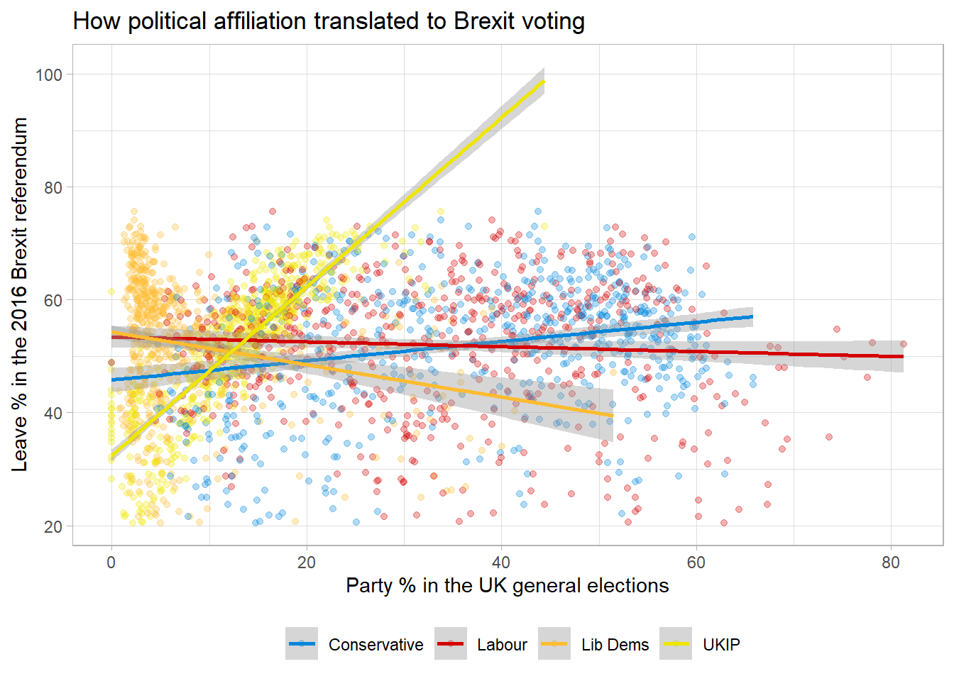

Looking at the graph, one may observe that the more the county is affiliated with UKIP, the more likely they are to vote for leave. The line is quite steep, which makes us think that the two variables are indeed correlated. Conversely, the more the country is affiliated with Liberal Democrats party, the more likely the citizens are to vote agains Brexit.

ggplot(brexit_results, aes(x = born_in_uk, y = leave_share)) +
  geom_point(alpha=0.25) +
  geom_smooth(method = "lm", col='#FFC0CB') +
  theme_minimal() +
  labs(title = "People born in UK scared of immigration?",
x = " Percent of UK Resident Born in the UK",
y = " Percent of votes cast in favor of Brexit ")

## `geom_smooth()` using formula 'y ~ x'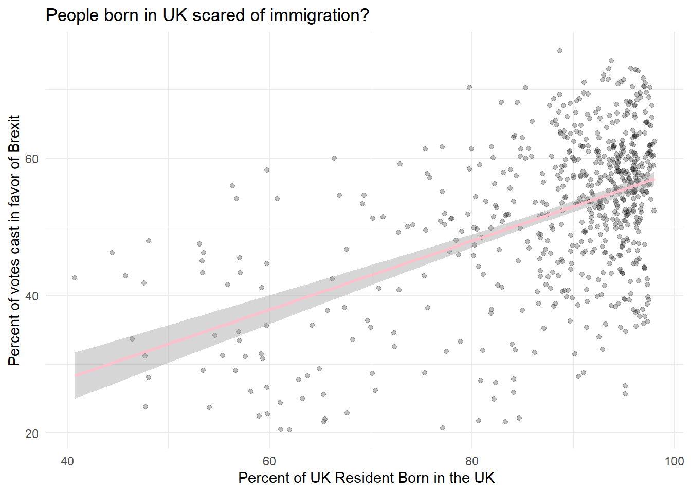

We can notice a high concetration of votes in the upper right corner, telling us that in the counties with high percentage of people born in the UK, there was a high percentage of votes in favor of Brexit.

sum(is.na(brexit_results$degree)) #Checking if there are any missing values

## [1] 59

degree_brex<-brexit_results %>% 
  filter(degree!= "NA") #filter for non missing values
  
  
hey<-ggplot(degree_brex, aes(x = degree, y = leave_share)) +
  geom_point(alpha=0.2) +
  #add pink regression line
  geom_smooth(method = "lm", col='#FF1493') +
  #change theme
  theme_minimal() +
  #add labels
  labs(title = "More people without a degree voted for Brexit!",
x = " Percent of UK Residents in a County Having a Degree",
y = " Percent of votes cast in favor of Brexit ", 
source= "https://www.thecrosstab.com/")

hey

## `geom_smooth()` using formula 'y ~ x'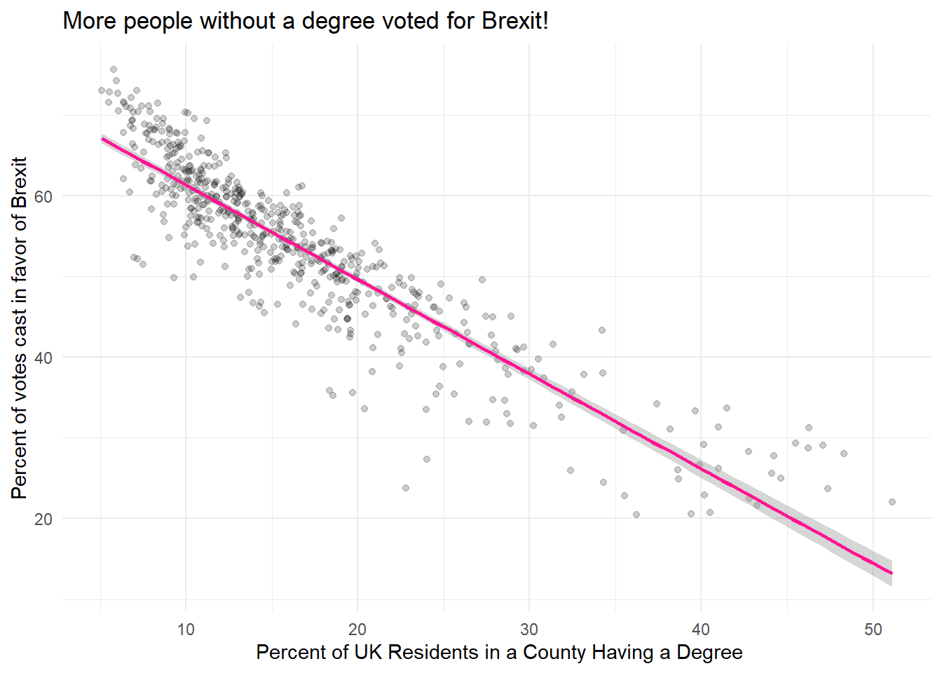

We can thus infer that conties lower percentages of degree votes for Brexit more, as the line sharply decreses when the percentage of degrees increses. If only the people were more educated so Brexit would not have happened!